Parameter learning and updates in simple word2vec
A lot of materials on word2vec models such as Skipgram and CBOW are available that explain the models really well. This post is just a drop in that ocean trying to clarify some of the details that I found useful in understanding the internals and explaining the models in line with the (almost the same) terminology used in the NLP lectures CS224n.Two other resources that I find very useful are word2vec Parameter Learning Explained and word2vec Explained: deriving Mikolov et al.’s negative-sampling word-embedding method.
A single training example (center-word, outside-word) pair
We first consider the simple case of predicting one outside word (outside word is a different terminology used in the lecture specfying a word in context of the input word) given a center word (the input word), i.e, the case for a single training sample.
As an example, consider the sentence “I love \(\underline{deep}\) learning NLP”. Lets consider window size of 5 and center word “deep”, so that the valid outside words are “I”, “love”, “learning” and “NLP”. So one training sample will constitute the pair, say (“deep”, “NLP”).
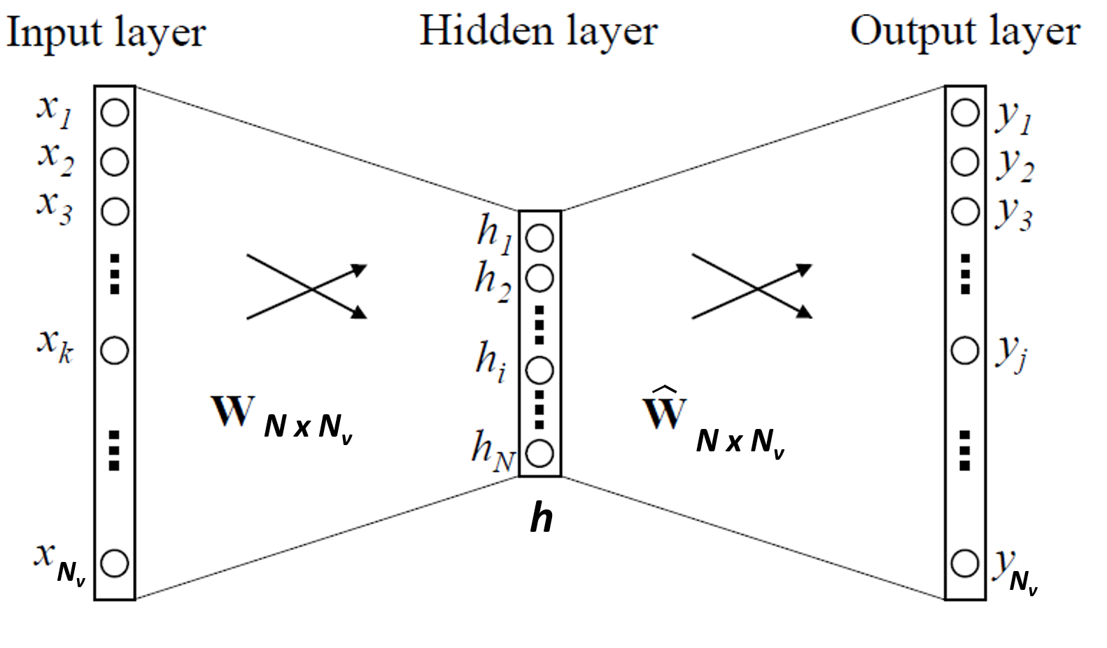
The word2vec model in figure below will learn the word embeddings while learning to predict a single outside word given a center word as input. Let \(\textbf{V} = \{w_1,w_2,...,w_{N_{\textbf{V}}} \}\) be the vocabulary. Here \(N_{\textbf{V}}\) is the number of words in \(\textbf{V}\).
Assume that the input center word occupies index \(c\), i.e, \(w_c\) in \(\textbf{V}\). Also assume that the “correct” output “outside” (context) word occupies index \(o\), i.e, \(w_o\) in \(\textbf{V}\). Let the input word is on-hot encoded as \(\textbf{x} = \{x_1,x_2,...,x_{N_{\textbf{V}}} \}\). Let the dimension of the word embeddings be \(N\). A single training sample constitutes the pair \((w_c,w_o)\) both one-hot encoded.
| Model with one center word and one outside word |
|---|
 |
The model will learn two vector representations for each word represented by the two matrices \(\textbf{W}\) and \(\hat{\textbf{W}}\).
The matrix \(\textbf{W}\) is the input-to-hidden layer weight matrix, has dimensions \(N \times N_{\textbf{V}}\). Column \(j\) of \(\textbf{W}\) denoted by \(\textbf{v}_j\) is the \(N\) dimensional vector representation of \(j\)th word in the vocabulary (\(w_j\)) when the word is used as center word. So the vector representation of the input word \(w_c\) is the \(c^{th}\) column \(\textbf{v}_c\) of \(\textbf{W}\).
Similary, the matrix \(\hat{\textbf{W}}\) is the hidden-to-output layer weight matrix, and also has dimensions \(N \times N_{\textbf{V}}\). Column \(j\) of \(\hat{\textbf{W}}\) denoted by \(\hat{\textbf{v}}_j\) is the \(N\) dimensional vector representation of \(j^{th}\) word in the vocabulary (\(w_j\)) when the word appears as outside (i.e context word) of another center word.
Given the input \(\textbf{x}\), the operation \(\textbf{Wx}\) produces the \(N\)-dimensional vector \(\textbf{h}\). That is, \(\textbf{h} = \textbf{Wx}\). But because \(\textbf{x}\) is one-hot encoding of \(w_c\), it has only the \(c^{th}\) position as 1 (and rest are 0’s), so \(\textbf{h}\) is simply the \(c^{th}\) column of \(\textbf{W}\). That is \(\textbf{h} = \textbf{Wx} = \textbf{v}_c\) (column vector of dimension \(N\)). So this is simply pulling out the vector representation of the center word from that matrix \(\textbf{W}\).
From the hidden layer to the output layer, the other weight matrix \(\hat{\textbf{W}}\) is used, which is also an \(N \times N_{\textbf{V}}\) matrix. Using these weights, we can compute a score \(u_j\) for each word \(w_j\) in the vocabulary: \(u_j = {\hat{\textbf{v}}_j}^{T} \textbf{h} = {\hat{\textbf{v}}_j}^{T} \textbf{v}_c\). That is, using matrix multiplication, \(\textbf{u} = \hat{\textbf{W}}^T \textbf{h}\), \(\textbf{u}\) is a \(N_{\textbf{V}} \times 1\) column vector.
Next we convert the raw scores \(u_j\) to probabilities using softmax,
\[y_j = \dfrac{\exp({u_j})}{\sum_{t=1}^{N_{\textbf{V}}} \exp(u_t)} = \dfrac {\exp( {\hat{\textbf{v}}_j}^{T} {\textbf{v}}_c ) } {\sum_{t=1}^{N_{\textbf{V}}} \exp({\hat{\textbf{v}}_t}^{T} {\textbf{v}}_c)} = P(w_j \vert w_c)\]When \(j=o\), the correct index of the outside word, \(y_j = y_o = p( w_o \vert w_c)\). Now we want to maximize the probability for the correct outside word prediction, i.e. \(p(w_o \vert w_c)\), or, the log of it (the likelihood),
\[\begin{align} \log(p(w_o \vert w_c)) &= {\hat{\textbf{v}}_o}^{T} {\textbf{v}}_c - \log( {\sum_{t=1}^{N_{\textbf{V}}} \exp({\hat{\textbf{v}}_t}^{T} {\textbf{v}}_c)} ) \\\\ & = -E \end{align} \tag{1}\]Here, \(E = - \log(p(w_o \vert w_c)) = - {\hat{\textbf{v}}_o}^{T} {\textbf{v}}_c + \log( {\sum_{t=1}^{N_{\textbf{V}}} \exp({\hat{\textbf{v}}_t}^{T} {\textbf{v}}_c)} )\) is the cross-entropy loss function (we want to minimize \(E\) ), and \(o\) is the index of the correct outside word in the output layer.
Update equations for vectors in \(\hat{\textbf{W}}\)
Taking the gradient of \(E\) w.r.t \(\hat{\textbf{v}}_o\) gives,
\[\frac{\partial E}{\partial \hat{\textbf{v}}_o} = -{\textbf{v}}_c + \dfrac {\exp( {\hat{\textbf{v}}_o}^{T} {\textbf{v}}_c ) } {\sum_{t=1}^{N_{\textbf{V}}} \exp({\hat{\textbf{v}}_t}^{T} {\textbf{v}}_c)} {\textbf{v}}_c = [p(w_o \vert w_c) - 1] {\textbf{v}}_c\]And for \(j \neq o\),
\[\frac{\partial E}{\partial \hat{\textbf{v}}_j} = [p(w_j \vert w_c) - 0] {\textbf{v}}_c\]So for all indices \(j\) which does not correspond to the correct outside word \(w_o\), using stochastic gradient descent with learning rate \(\eta\), the weight updating equations for hidden-to-output weight vector \(\hat{\textbf{v}}_j\) is,
\({\hat{\textbf{v}}_j}^{(new)} = {\hat{\textbf{v}}_j}^{(old)} - \eta [p(w_j \vert w_c) - 0] {\textbf{v}}_c = {\hat{\textbf{v}}_j}^{(old)} - \eta [p(w_j \vert w_c) - 0] \textbf{h}\).
Intuitively, update \(\hat{\textbf{v}}_j\) if \(p(w_j \vert w_c) \gt 0\) (over-estimation, subtract a fraction of \(\textbf{h}\) from \(\hat{\textbf{v}}_j\)).
And for the vector \(\hat{\textbf{v}}_o\) (for the correct output word \(w_o\)), the update is
\({\hat{\textbf{v}}_o}^{(new)} = {\hat{\textbf{v}}_o}^{(old)} - \eta [p(w_o \vert w_c) - 1] {\textbf{v}}_c = {\hat{\textbf{v}}_o}^{(old)} - \eta [p(w_o \vert w_c) - 1] \textbf{h}\).
Intuitively, update \(\hat{\textbf{v}}_o\) if \(p(w_o \vert w_c) \lt 1\) (under-estimation, add a fraction of \(\textbf{h}\) to \(\hat{\textbf{v}}_o\)).
Thus each column of \(\textbf{W}\) will be updated using the above two equations for a single training example.
Update equations for vectors in \(\textbf{W}\)
Taking the gradient of \(E\) w.r.t \(\textbf{v}_c\) gives,
\(\frac{\partial E}{\partial {\textbf{v}}_c} = -{\hat{\textbf{v}}}_o + \sum_{t=1}^{N_{\textbf{V}}} \lbrace \dfrac {\exp( {\hat{\textbf{v}}_t}^{T} {\textbf{v}}_c ) } {\sum_{k=1}^{N_{\textbf{V}}} \exp({\hat{\textbf{v}}_k}^{T} {\hat{\textbf{v}}}_t)} \rbrace {\hat{\textbf{v}}}_t = \sum_{t=1}^{N_{\textbf{V}}} p(w_t \vert w_c) {\hat{\textbf{v}}}_t - {\hat{\textbf{v}}}_o\).
And, for any column \(j \neq c\), clearly, \(\frac{\partial E}{\partial {\textbf{v}}_j} = 0\). So only for vector \(\textbf{v}_c\) (\(c^{th}\) column of \(\textbf{W}\), we will have an update,
\({\hat{\textbf{v}}_c}^{(new)} = {\hat{\textbf{v}}_c}^{(old)} - \eta \frac{\partial E}{\partial {\textbf{v}}_c}\). No updates for any other columns in \(\textbf{W}\).
Update equations for all (center-word, outside-word) pairs from the corpus
Coming soon WTP.
