Denoising Images using Ising model
This post develops on the Ising model concepts from my previous blog, see Ising model. Consider the problem of reconstructing a black-and-white image (i.e. each pixel is either 1 or -1) from the corrupted observations. We assume that there is an underlying (hidden) noise-free image from which the observed image (Figure 1) is generated by adding noise: randomly flip the pixel values with a small probability (say 20%). Given the observed noisy image (modeled by random variable \(\textbf{Y}\)), we want to recover the original noise-free image (modeled by random variable \(\textbf{X}\).
| Noise-Free Image | Noisy Image |
|---|---|
 |
 |
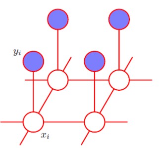
Consider the figure of an undirected graphical model representing a Markov random field for image de-noising (taken from Bishop’s book.  . \(x_i\) is a binary variable denoting the state of pixel \(i\) in the unknown noise-free image, and \(y_i\) denotes the corresponding value of pixel \(i\) in the observed noisy image.
So we have \( \textbf{X} =\{ X_1,X_2,…,X_n \} \) as our hidden random variables (corresponding to the unobserved noise-free image) on set \( S=\{1,2,…,n\} \) of pixels (or sites). And, \( \textbf{Y} =\{ Y_1,Y_2,…,Y_n \} \) as our observed random variables (corresponding to the observed noisy image). Each \(X_i\) is binary, i.e, \(X_i\) takes value \(x_i \in L=\{-1,1\}\). Similarly for \(Y_i\).
Assume a clumpy model with higher correlations between a \(X_i\) with its neighbors, say \(X_j\) than between \(X_i\) and \(Y_i\). We want to infer \(X\) that maximizes the probability \(P(X \vert Y) = \dfrac{P(Y \vert X)P(X)}{P(Y)}\). Here, \(P(Y \vert X)\) is the liklihood and \(P(X)\) is the prior. Now, we will use the Ising model as the prior \(P(X)\), as
\[P(X) = \dfrac{1}{Z}\exp\{ -U(\textbf{x}) \} = \dfrac{1}{Z}\exp\{ -\alpha\sum\limits_{\{i\} \in C_1} x_i + \beta\sum\limits_{\{i,j\} \in C_2} x_i x_j\}\]Assume that the pixels in the noise-free image are corrupted by an indepedent zero-mean Gaussian noise, i.e,\(y_i = x_i + \epsilon_i\) where \(\epsilon_i\) is \(N(0,\sigma^2)\) iid. Then, \(P(y_i \vert x_i) = \dfrac{1}{\sqrt{2 \pi {\sigma}^2}}exp\{ -\dfrac{(y_i-x_i)^2}{2{\sigma}^2}\}\), so that the full joint model becomes \(P(\textbf{Y} \vert \textbf{X}) = (\dfrac{1}{\sqrt{2 \pi {\sigma}^2}})^n exp\{ -\dfrac{\sum_{i=1}^n (y_i-x_i)^2}{2{\sigma}^2}\}\).
We will sample from the posterior \(P(X \vert Y)\) using Gibb’s sampling (as we did in Ising Model and then use the mean of the samples from the posterior as an estimate of the denoised image. We have
\[\begin{align} P(\textbf{X}|\textbf{Y}) & = \dfrac{P(\textbf{Y|X}) P(\textbf{X})}{P(\textbf{Y})} \\\\ & = \dfrac{1}{P(\textbf{Y})} \underbrace{[(\dfrac{1}{\sqrt{2 \pi {\sigma}^2}})^n \exp\{ -\dfrac{\sum_{i=1}^n (y_i-x_i)^2}{2{\sigma}^2}\}] [\dfrac{1}{Z}\exp\{ -\alpha\sum\limits_{\{i\} \in C_1} x_i + \beta\sum\limits_{\{i,j\} \in C_2} x_i x_j\}}_{P(\textbf{X,Y})} ] \\\\ & = \dfrac{1}{P(\textbf{Y})} \dfrac{1}{Z} (\dfrac{1}{ \sqrt{2 \pi {\sigma}^2}})^n \exp\{ -\dfrac{\sum_{i=1}^n (y_i-x_i)^2}{2{\sigma}^2} -\alpha\sum\limits_{\{i\} \in C_1} x_i + \beta\sum\limits_{\{i,j\} \in C_2} x_i x_j\} \end{align}\]Now to do Gibb’s sampling, we need \(P(x_i \vert N(x_i))\), where \(N(x_i)\) now include \(y_i\) as well because now there is an edge between \(x_i\) and \(y_i\).
From Gibb’s sampling in Ising Model, \({P(x_i,N(x_i))} = \dfrac{P(x_i,N(x_i))}{P(x_i=-1,N(x_i)) + P(x_i=1,N(x_i))}\).
Therefore, \({P(x_i=1\vert N(x_i))} = \dfrac{\exp\{ -\dfrac{\sum_{i=1}^n (y_i-1)^2}{2{\sigma}^2} -\alpha + \beta\sum\limits_{x_j \in N(x_i)} x_j\}} { \exp\{ -\dfrac{\sum_{i=1}^n (y_i-1)^2}{2{\sigma}^2} -\alpha + \beta\sum\limits_{x_j \in N(x_i)} x_j\} + \exp\{ -\dfrac{\sum_{i=1}^n (y_i+1)^2}{2{\sigma}^2} +\alpha - \beta\sum\limits_{x_j \in N(x_i)} x_j\} }\).
And, \({P(x_i=-1\vert N(x_i))} = 1 - {P(x_i=1\vert N(x_i))}\).
A python implementation is at github.
